Transformation Nodes

The various transformations that can be performed on a source are explained in this section.

Following are the steps to perform transformation:

Drag and drop the node from the Transformation section to the pipeline editor page.
Connect the source node to the transformation node.
Double-click the transformation node. The properties of the node will be displayed. For more details, see the Node Settings section.
Configure the properties and save the settings. The properties for each node are explained in the following sections.

NOTE: After you configure the node properties and click Data, sometimes the required data might not be fetched, or fetching data might take an unusually longer time. This is mainly due to network issues. To resolve such issues, see the Configuring Data Validation in Node Properties section.

Filter

The Filter transformation node allows you to filter the required data/columns from the connecting source table or other nodes.

Following are the steps to apply Filter node in pipeline:

Double-click the Filter node. The properties page is displayed.
Click Add Filter, enter the required values and click Save.

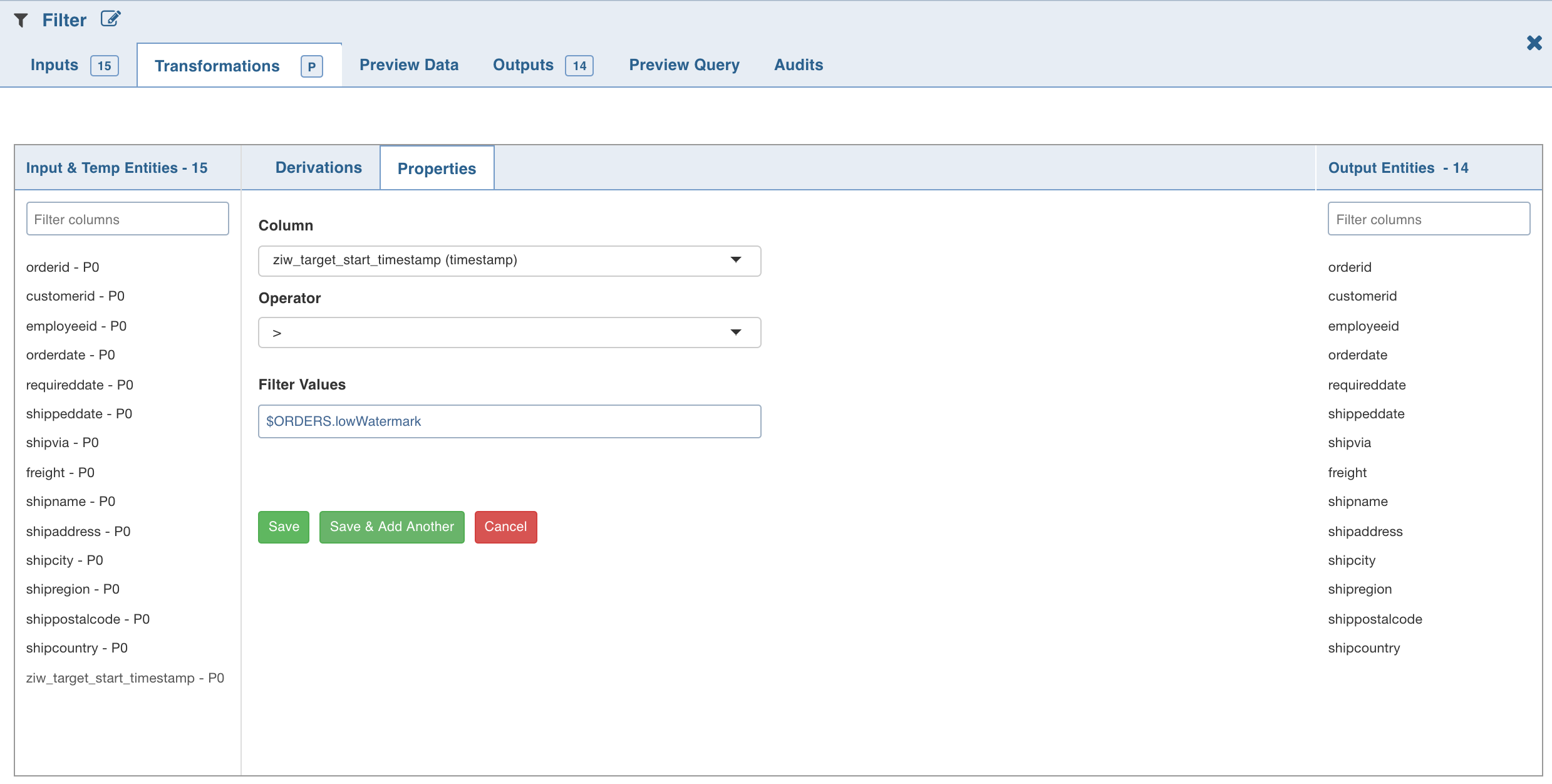
The added filters will be listed in the Properties section. The Properties section with the low and high watermark values will be displayed.

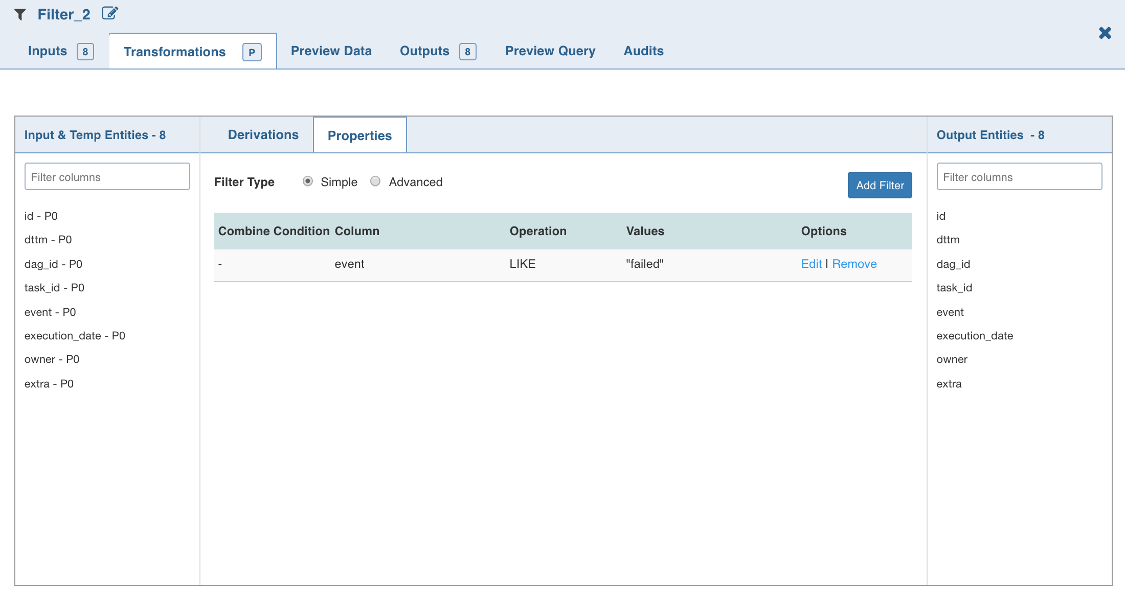
To add SQL filter query, select Advanced filter type and click Edit Filter.
Enter the SQL query and click OK.

Join

The Join node allows you to join two or more tables/nodes.

Following are the steps to apply Join node in pipeline:

Double-click the Join node. The properties page is displayed.

Select the Left Port (main table). All the other tables will have one or more join conditions with the left table.
Click Edit Join , enter the required values and click Save.

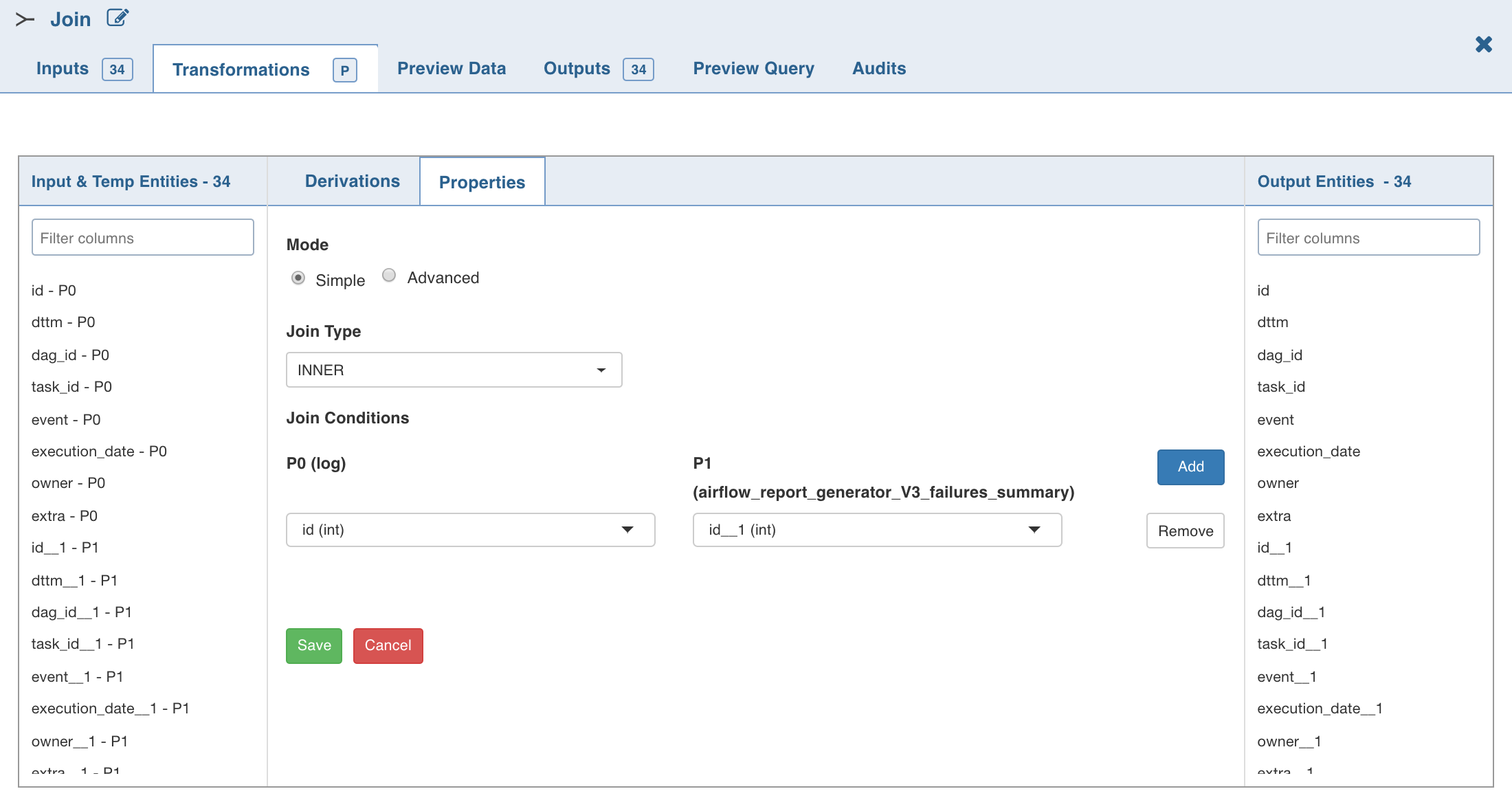
To set the join expression, select Advanced mode and enter the join expression and click Save. A sample expression is explained below:

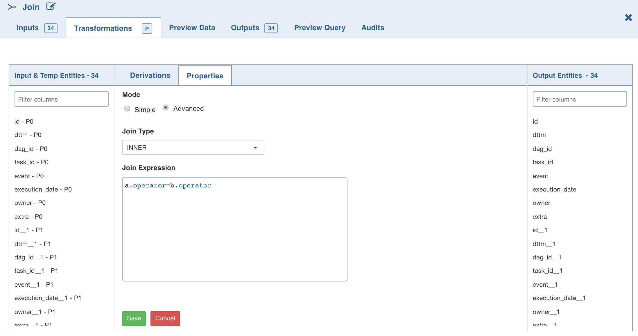
Here, a and b are node names and ORDERID is the column name from corresponding nodes.

NOTE: Disjuncts, Relational operators other than equals (=), and Complex join conditions (like column1+column2 = 100) are not supported.

The join node creates a new result table by combining columns from multiple tables.

Inner Join: Returns all the rows where the selected columns from left and right tables match.
Left Outer Join : Creates a new result table which returns all the rows in the left table and only those rows in the right table where the selected column values of left and right tables match.
Right Outer Join : Creates a new result table which returns all the rows in the right table and only those rows in the left table where the selected column values match.
Full Outer Join : Creates a new result table which returns the intersecting rows joined together, as well as the non-intersecting rows from both tables, with null values for fields of the other table.
Cross Join : Produces a cross product of two tables. The number of records in the resulting table is equal to the number of rows in the left table multiplied by the number of rows in the right table. This does not require any join condition.

The join conditions are validated and added to the read-only view. Errors if any, will be displayed at the top of the transformation page.

NOTE: If the column names of the incoming nodes match with the ones in the connecting nodes, the column name of the connecting node automatically changes with a few extra characters suffixed to the name. This is to avoid conflicts in the column names. Internally, column references are stored to track lineage and global search. You can change the column names if required. The same column rename functionality flow will be followed.

Even after renaming a column in the Schema section, the original column name will be shown in the Properties window. However, the renamed column will be propagated in the downstream nodes.

For spark execution engine, to use join node and cross join between any two columns, the spark.sql.crossJoin.enabled configuration must be set to true in the spark configuration file.

Post Processing Configuration

Post processing configuration allows you to dynamically partition the output of a node for subsequent node processing. It includes the Repartitioning and Sorting options.

NOTE: This feature is available only for Spark.

Repartitioning

You can navigate to Configurations > Edit Configurations page and select Enable Repartitioning (repartitioning is optional). The following page is displayed.

You can select a list of columns. The columns with unique values will be partitioned into a single set. For this subsequent downstream node, processing will be faster based on the partitioned data. You can select any column which is a part of Outputs.

Sorting

Once data is partitioned, you can sort the data in the columns within the partition. This enables faster data access and data processing in downstream nodes.

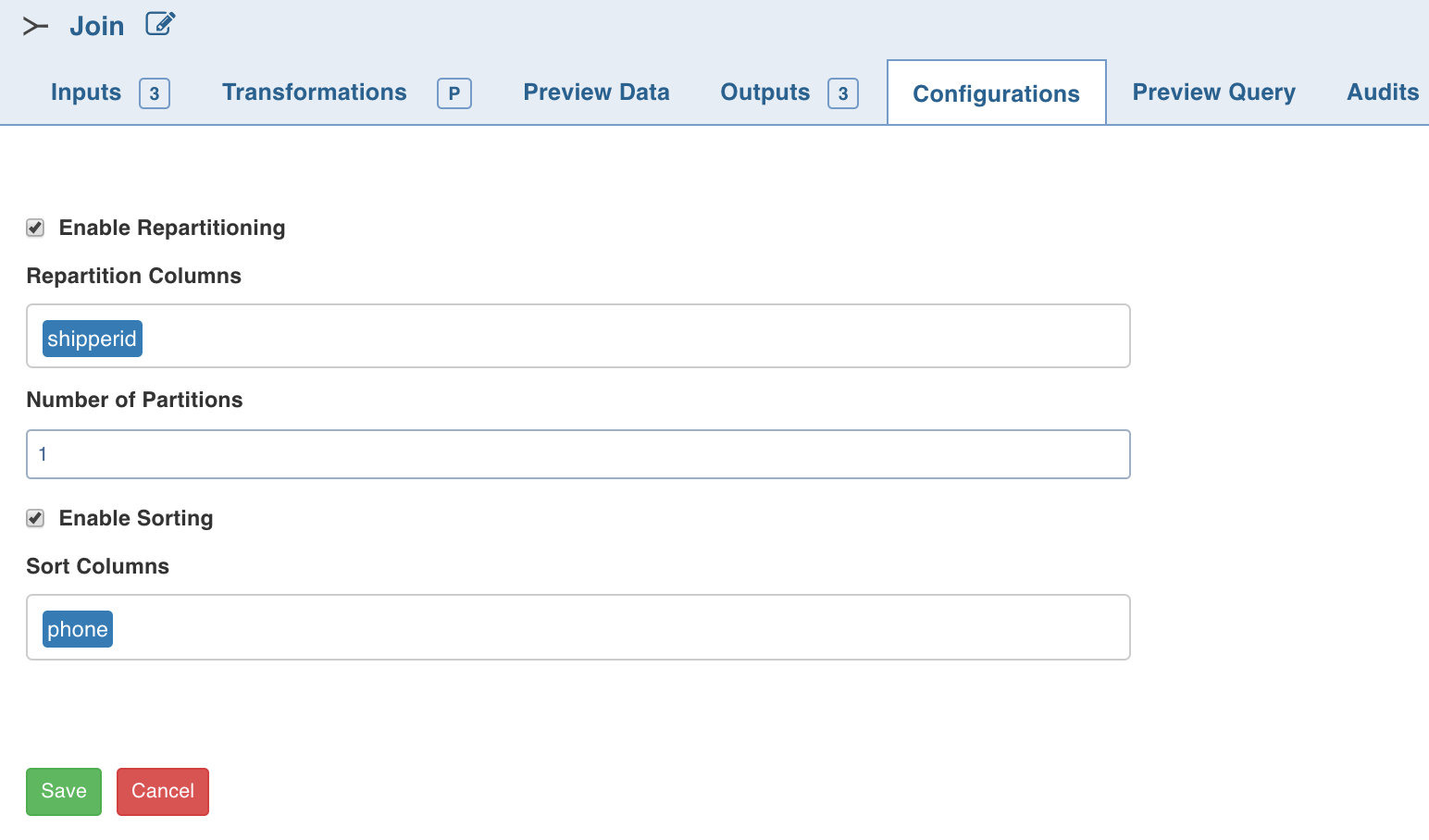
NOTE: Columns selected for repartition cannot be used for sorting.

Broadcast Join

NOTE: This feature is available only for Spark execution engine.

Spark SQL uses Broadcast Join (Broadcast Hash Join) instead of Hash Join to optimize join queries when the size of one side data is below the spark.sql.autoBroadcastJoinThreshold value.

Broadcast join can be efficient for joins between a large table (fact) with relatively small tables (dimensions) that could then be used to perform a star-schema join. This avoids sending all data of the large table over the network.

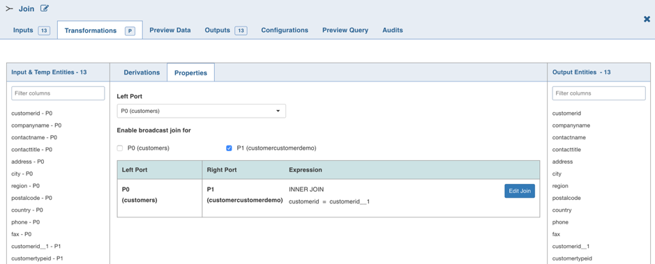
Following are the steps to enable Broadcast join for the join node in pipeline:

Double-click the Join node. The properties page is displayed.
Select the port for which broadcast join is required. The selection will be autosaved.

The selected port(s) will be broadcasted when the execution occurs.

Derive

The Derive node allows you to derive one or more columns from the node joined to this node on the pipeline.

Following are the steps to apply Derive node in pipeline:

Double-click the Derive node.
Click Add Derivation, enter the required details and click Save.

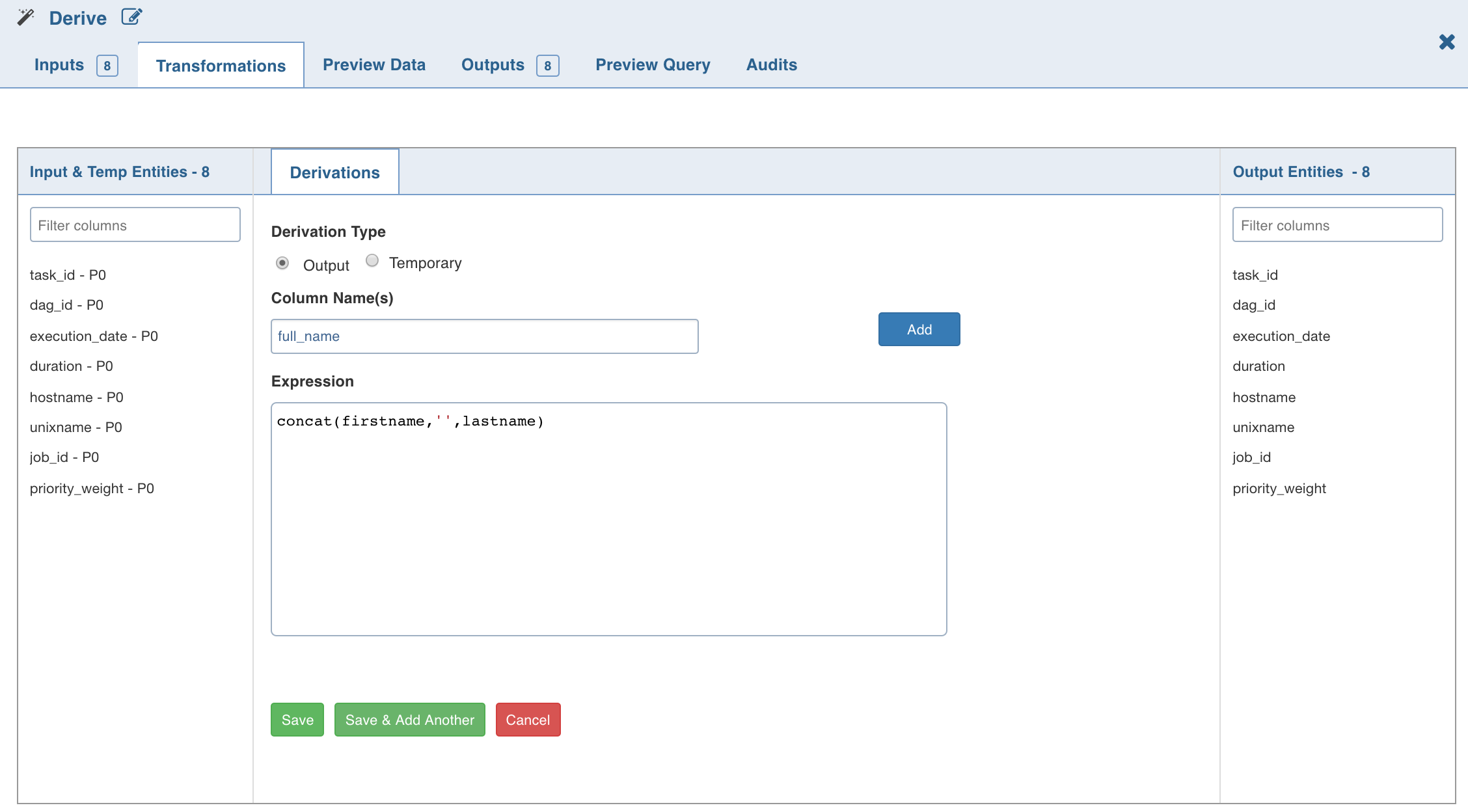
NOTE: The expression can include any of the operators, non-aggregation functions and advanced analytics functions supported by Data Transformation. The expression gets validated for syntax and semantic errors, and any error message is displayed on the top of the page.

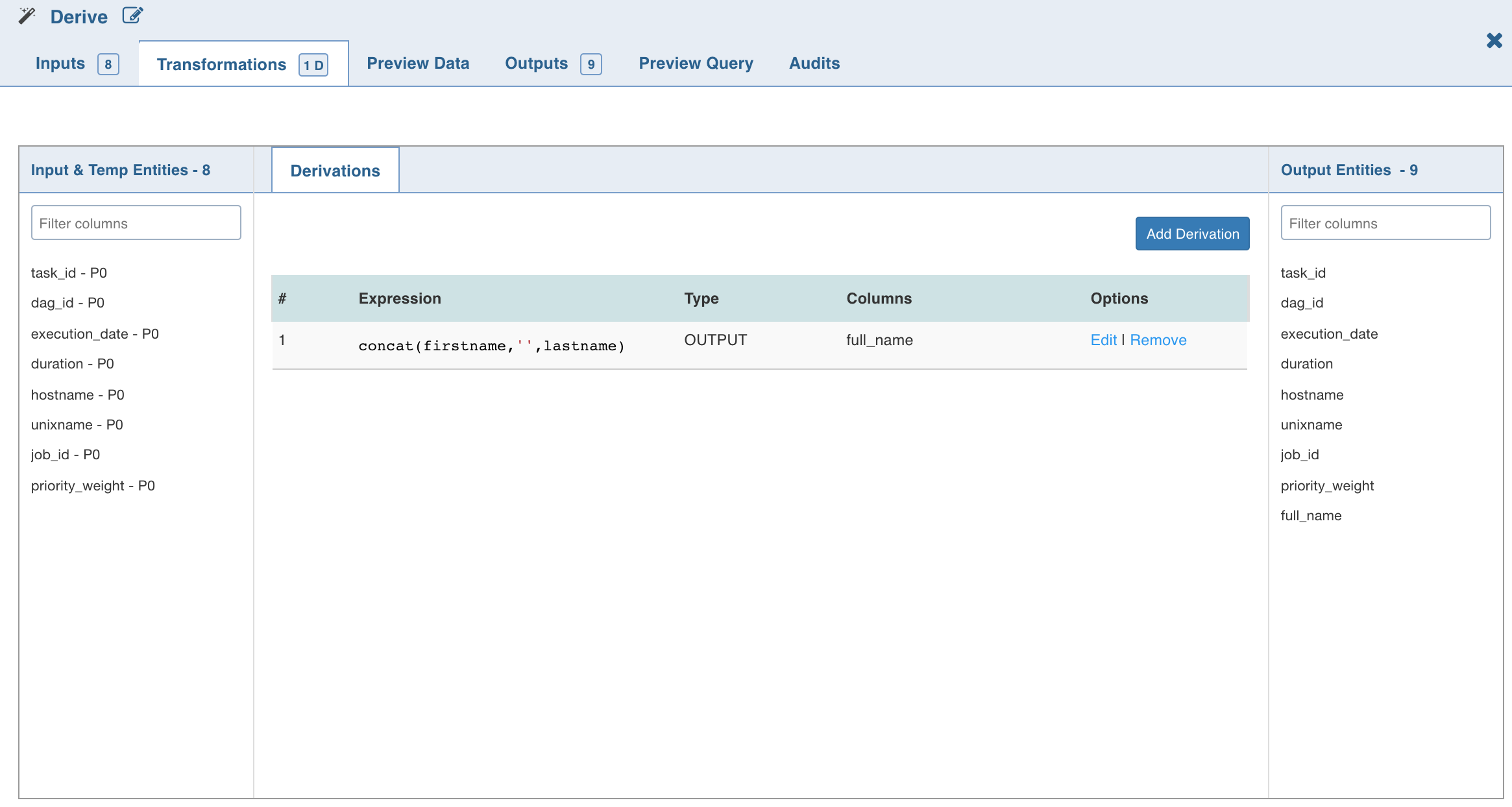
The Derive properties page with the derived column and expression added is as follows:

Aggregate

The Aggregate node allows you to derive new columns by applying aggregate functions such as, count, distinct count, sum, distinct sum, min, max, average, distinct average, and variance over a group of values.

Following are the steps to apply Aggregate node in pipeline:

Double-click the Aggregate node. The properties page is displayed.
Click Add Group By, select the column for which the derived data is to be grouped by, and click Save.

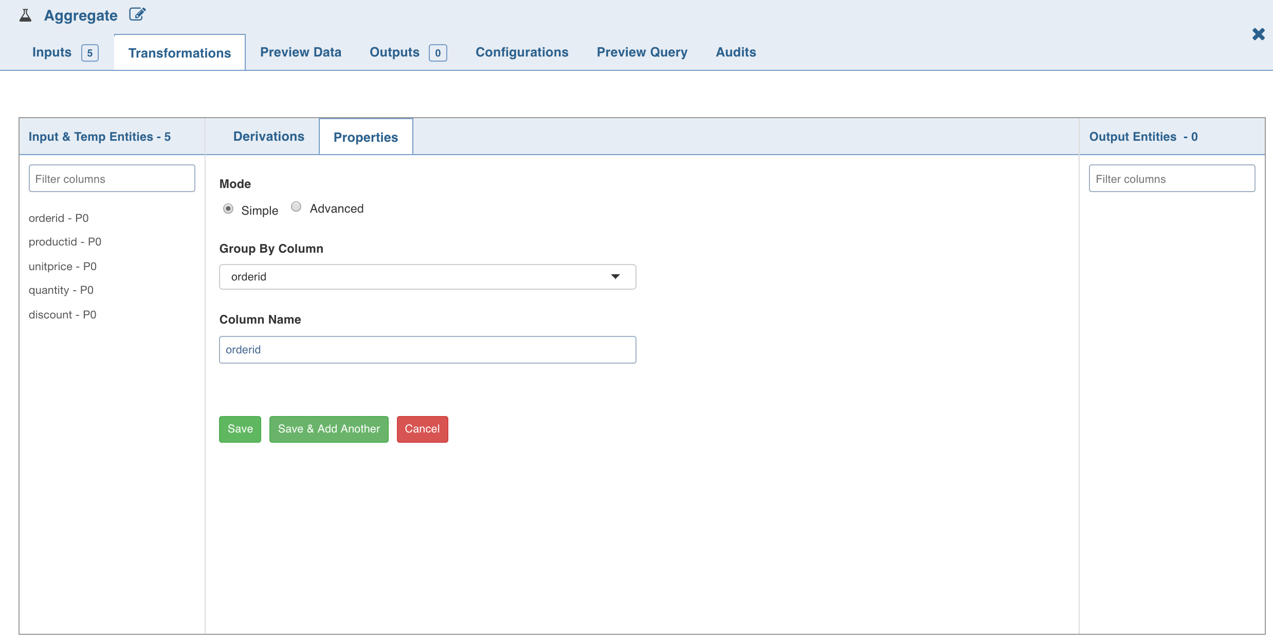
To set the expression, select Advanced mode and enter the expression and click Save.
Click Add Aggregate. The following page is displayed.

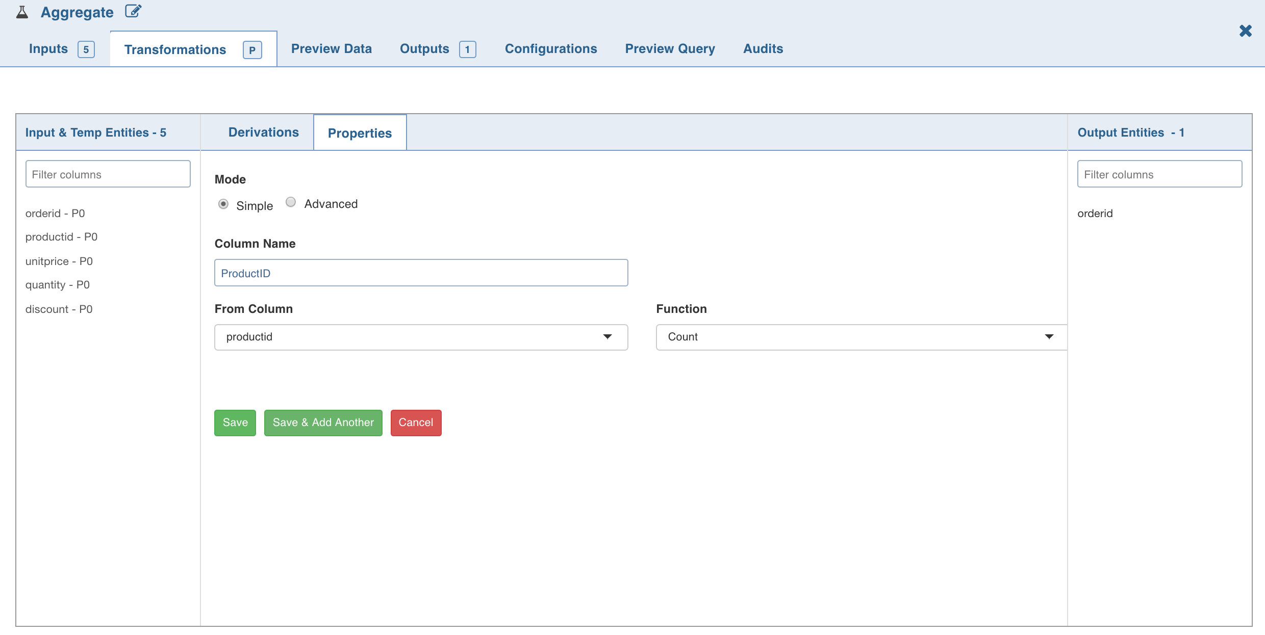
NOTE: For columns that include integers and dates as datatypes, all the functions will be enabled in the Function drop-down list. For the columns that have strings as datatypes, only Count and Distinct Count functions will be enabled.

To set the Aggregate expression, select Advanced mode and enter the expression and click Save. The aggregated data is fetched based on the columns and functions used. All group by and derived columns are added in the metadata section.

Post Processing Configuration

Post processing configuration allows you to dynamically partition the output of a node for subsequent node processing. It includes the Repartitioning and Sorting options.

It includes Repartitioning and Sorting options.

Repartitioning

You can navigate to Configurations > Edit Configurations page and select Enable Repartitioning (repartitioning is optional). The following page is displayed:

Sorting

Once data is partitioned, you can sort the data in the columns within the partition. This enables faster data access and data processing in downstream nodes.

NOTE: Columns selected for repartition cannot be used for sorting.

Distinct

Distinct node allows you to retrieve distinct values/rows in a table.

Duplicate records in a data set must be removed before data mining. For example, in a marketing database, individuals may appear multiple times with different address or company information. You can use the Distinct node to find, or remove, duplicate records in your data set. Distinct node starts with zero rows and columns.

Following are the steps to retrieve only the distinct rows in a table:

Double-click the Distinct. The Properties page is displayed.
Click Add Distinct, enter the required details and click Save.

The Distinct Properties page is displayed. You can verify the content in Schema and Data sections.

Post Processing Configuration

Post processing configuration allows you to dynamically partition the output of a node for subsequent node processing. It includes the Repartitioning and Sorting options.

It includes Repartitioning and Sorting options.

Repartitioning

Navigate to Configurations > Edit Configurations and select Enable Repartitioning (repartitioning is optional). The following page is displayed.

Sorting

Once data is partitioned, you can sort the data in the columns within the partition. This enables faster data access and data processing in downstream nodes.

NOTE: Columns selected for repartition cannot be used for sorting.

Union

Union node allows you to combine the data from two or more tables (nodes).

NOTE: Hive versions prior to 1.2.0 supports only UNION ALL and not UNION DISTINCT.

Following are the steps to apply Union node in pipeline:

Double-click the Union node. The properties page is displayed.
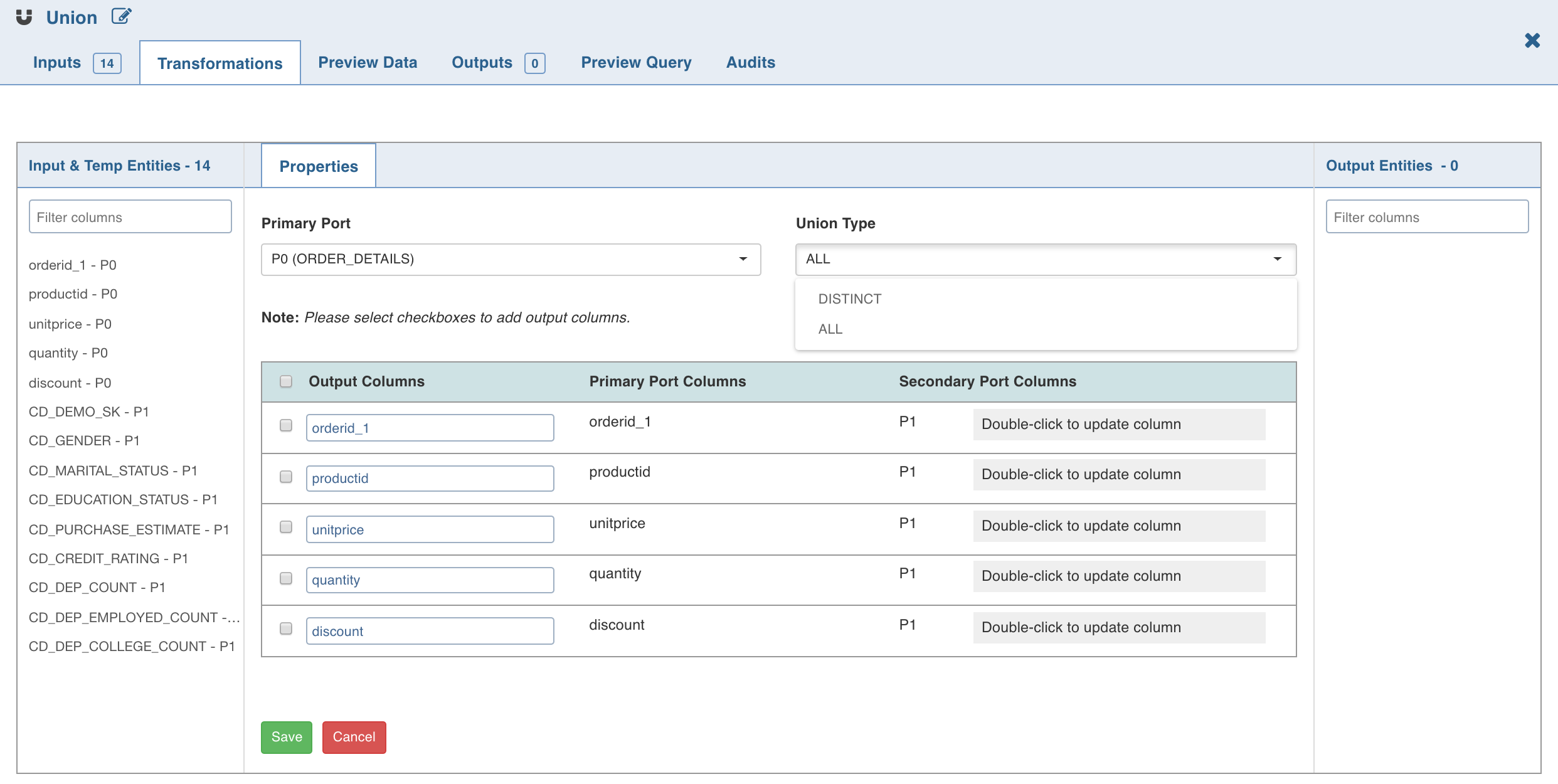
Click Edit Union to add union data. The tables (nodes) involved in the union condition are displayed along with column name section.

Select the following details and click Save:

Primary Port to which the rest of the tables will be combined.

NOTE: Columns of other tables can be mapped to the primary table. You cannot change the order of primary table columns. All the column fields in the other table sections can be edited depending on which columns of that table and the primary table should match. You can change the primary table using the primary table drop-down.

Type: The ALL option adds all the rows to the union node. DISTINCT adds only distinct rows to the union node.
If necessary, rename the columns under Column Name. The Column Name includes the columns of the Primary Table and only these names can be edited.
Map/rearrange the column order of the other tables (based on name) using edit. The edit feature is not available for primary tables.
Use the checkboxes on the left of primary table column names to add or remove the columns in the union node.

NOTE: When Using Impala as Execution Engine, UNION DISTINCT is not supported.

Known Issue

The changes made to the upstream nodes such as Aggregate and Distinct nodes, connecting to the Union node may not propagate into the Union node. Workaround: To have the changes propagated in the Union node, click Edit Union and remap it.

Split

Split node allows you to break up a multi-valued column into multiple rows with new columns which have a part of the value.

Following are the steps to apply Split node in pipeline:

Double-click the Split node. The properties window is displayed.
Click Add Split Column, enter the required details and click Save.

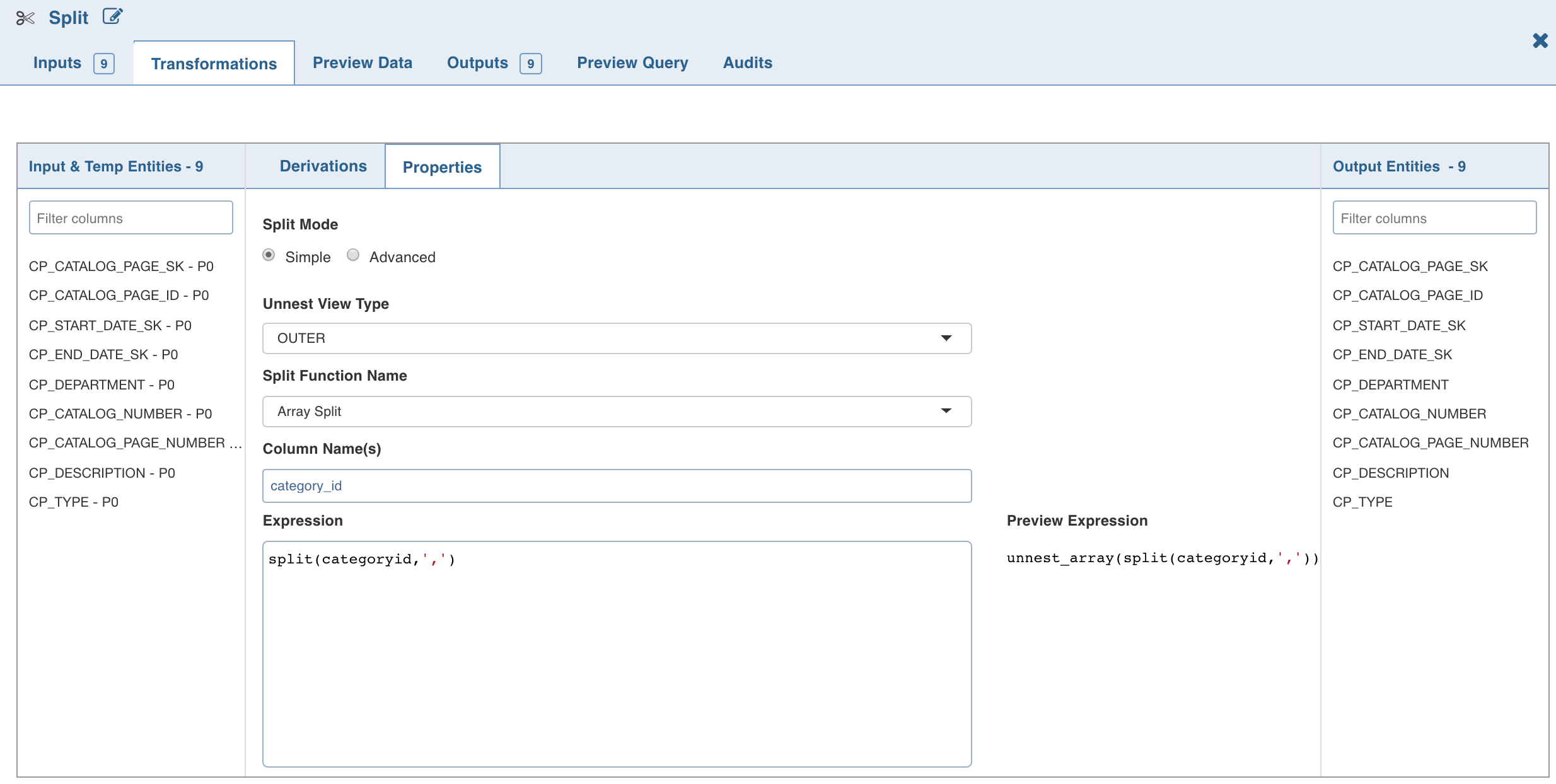
To set the split expression, select Advanced mode and enter the expression and click Save.

The Split transformation supports three functions:

Array Split
Array Split + Position
Map Split The following table describes the Split transformation functions in detail:

Function	New Columns	Example Expression	Example Output
Array Split	1 (value)	split('a,b,c',',')	a b c
Array Split with Position	2 (position, value)	split('a,b,c',',')	0 a 1 b 2 c
Map Split	2 (key, value)	str_to_map('k1:v1,k2:v2')	k1 v1 k2 v2

NOTE: The expression can use any of the operators and non-aggregation functions. The expression gets validated for syntax and semantic errors, and any error message is displayed on the top of the page.

The Split By operations are added in the Properties section as follows:

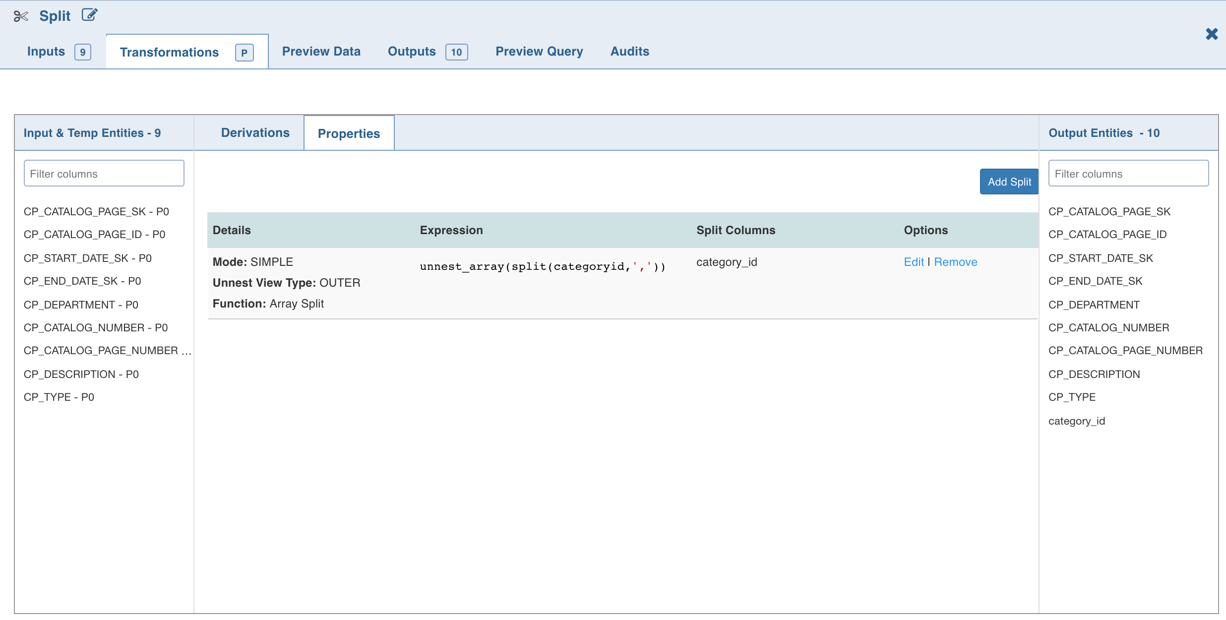
NOTE: The Split (say S1) created will not be available in the Inputs. To use S1 as a part of another split (say S2), follow the below steps:

Create an additional split node.

Link it to the existing split node.

S1 will now be displayed in the Inputs and can be used in S2.

Cleanse

The Cleanse node allows you to perform a column value cleaning or look up related data in a source, and return the data for use in downstream processing. To return many related records, the matching data is returned in array attributes. You can then choose to split this data (effectively creating a join across the working data and the Reference Data) using the Split node on these array attributes.

Following are the steps to apply Cleanse node in pipeline:

Double-click the Cleanse node. The properties page is displayed.
Click Add Transformation, enter the required details and click Save.

Following are the two types of Cleanse transformations:

Generic Lookup: In generic lookup transformation, you must select cleanup column and a lookup table. Based on the lookup table selection, drop-downs for lookup and value columns are displayed. Select the required lookup and value columns.
Lookup: In lookup transformation, you must select cleanup column and lookup table. You need not select lookup and value column. By default, the first and second columns will be considered as lookup and value columns respectively.

Lookup

Lookup node can be used to fetch column information (derived column) from the lookup source based on the rule that applies to each input record.

Following are the steps to apply Lookup node in pipeline:

Double-click the Lookup node. The properties page is displayed.

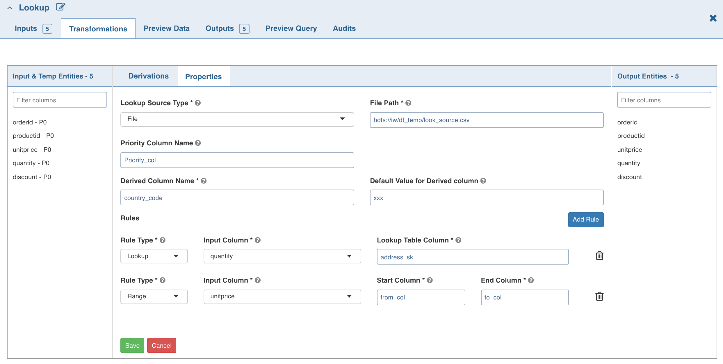
Enter the following details:

Lookup Source Types: The source types supported are File and Table.
File: If you select file, the File Path field is displayed. Provide the CSV file path.

NOTE: Ensure you provide absolute path of the CSV file.

Table: If you select table, the Schema Name and Table Name fields are displayed. Provide the Hive table details.

NOTE: A lookup record is matched only if all the rules (Range/Lookup) are satisfied (AND of all the rules).

Priority Column Name: Column that indicates the lookup record priority. In case of multiple matching lookup records, the record with the highest priority will be used.
Derived Column Name: Column which must be derived from the lookup table.
Default Value: Default value if no rule matches from the lookup table.
Rule Type: Lookup - to perform the exact value comparison with lookup column, Range - to perform the range comparison with lookup columns.
Input Column: The input column which must be compared against lookup column(s).
Lookup Table Column (Lookup rule): lookup table column which must be compared with given input column.
Start Column (Range rule): lookup table column which specifies start range for the specified input column.
End Column (Range rule): lookup table column which specifies end range for the specified input column.

Limitation

Currently, only non-overlapping ranges are supported.

Fuzzy Match

Transformation designers can now use a pre-built Fuzzy Matching transformation component to match and score similar data, by overcoming spelling, phonetic and other data quality issues.

Following are the steps to apply Fuzzy Match node in pipeline:

Double-click the Fuzzy Match node. The properties page is displayed.
Select the Input Port.
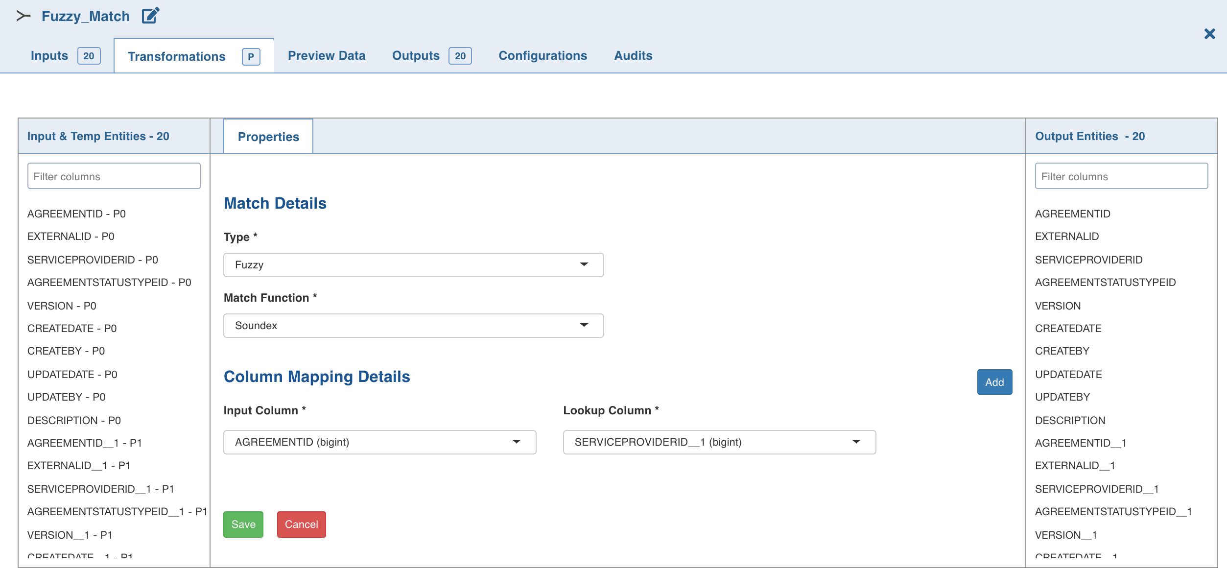
Click Add Match Property, enter the required details and click Save.

Properties

Type: A fuzzy node can have multiple match properties. For each match property, there can be multiple column mappings. The options include exact and fuzzy. Match property of type Exact performs inner join on the column mapping details provided.
Match Function: The fuzzy match function. The options include Soundex and Levenshtein.

Levenshtein returns a match score for the input and lookup tables. According to Levenshtein algorithm, lower the match score the better is the match.

The result dataset of Soundex contains only those values of the input and lookup column where the soundex algorithm returns true. Soundex accepts input port column and lookup port column only of type String.

Score Column Name: This field is displayed only if the match function selected is Levenshtein.
Threshold - High: This field is displayed only if the match function selected is Levenshtein. Indicates the high threshold to filter out the data higher than this threshold value. The data which satisfies the condition of lesser than or equal to the threshold value will be displayed.
Input Column: Input column that must be compared against lookup column.
Lookup Column: Lookup table column that must be compared with the given input column.

NOTE: The Soundex algorithm accepts columns of string type only.

In NotIn

The In NotIn node has two inputs: inner table and outer table. The outer table is the table to be filtered. Columns of only this node will be propagated downstream. The inner table is the filtering table.

A column of the outer table (outer column), will be matched against a column of the inner table (inner column) to filter records of the outer table.

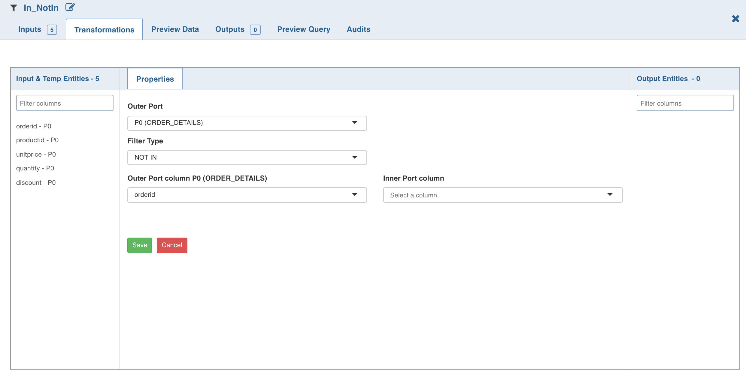
Selecting the IN filter type returns only those records from the outer table where the outer column value exists in the list of values in inner column. Selecting Not IN filter type returns only those records from the outer table where the outer column value does not exist in the list of values in inner column.

Following are the steps to apply In NotIn node in pipeline:

Double-click the In NotIn node. The properties page is displayed.
Click Add Filter, enter the required details and click Save.

NOTES:

The NOT-IN transformation produces an empty result, if the inner-column is nullable. This is because NOT IN is equivalent to <> ALL. If the inner column has a null, its comparison with any outer column value always produces null. Work-around: To obtain the required result, remove NULL values from inner-column by inserting a filter node (IS NOT NULL) between inner-table node and IN-NOTIN node.
Even after renaming a column in the Schema section, the original column name will be displayed in the Properties. However, the renamed column will be propagated in the downstream nodes.

Exists

The Exists node provides the functionality of correlated-subqueries in the where clause. It has two input tables/nodes, namely, inner table and outer table.

The outer table is the table to be filtered. Columns of only this node will be propagated downstream. The inner table is the filtering table and is used in the subquery-predicates.

A conjunction of subquery-predicates must be specified in the inner table expression text-box, with at least one correlated-subquery-predicate containing the equals (=) operator.

For correlated-predicates, one side of the equals (=) operator must reference at least one column from the outer table and the other side must reference at least one column from the inner table.

Selecting the EXISTS filter type returns only those records from the outer table where the subquery predicate evaluates to be true. Selecting the NOT EXISTS filter type returns only those records from the outer table where the subquery predicate evaluates to be false.

NOTE: Subqueries cannot contain windowing clauses and nested subqueries are not supported.

Following are the steps to apply Exists node in pipeline:

Connect two required nodes (outer and inner tables) to the Exists node.
Double-click the Exists node. The properties page is displayed.
Click Add Filter, enter the required details and click Save. The following is an example for inner table expression.

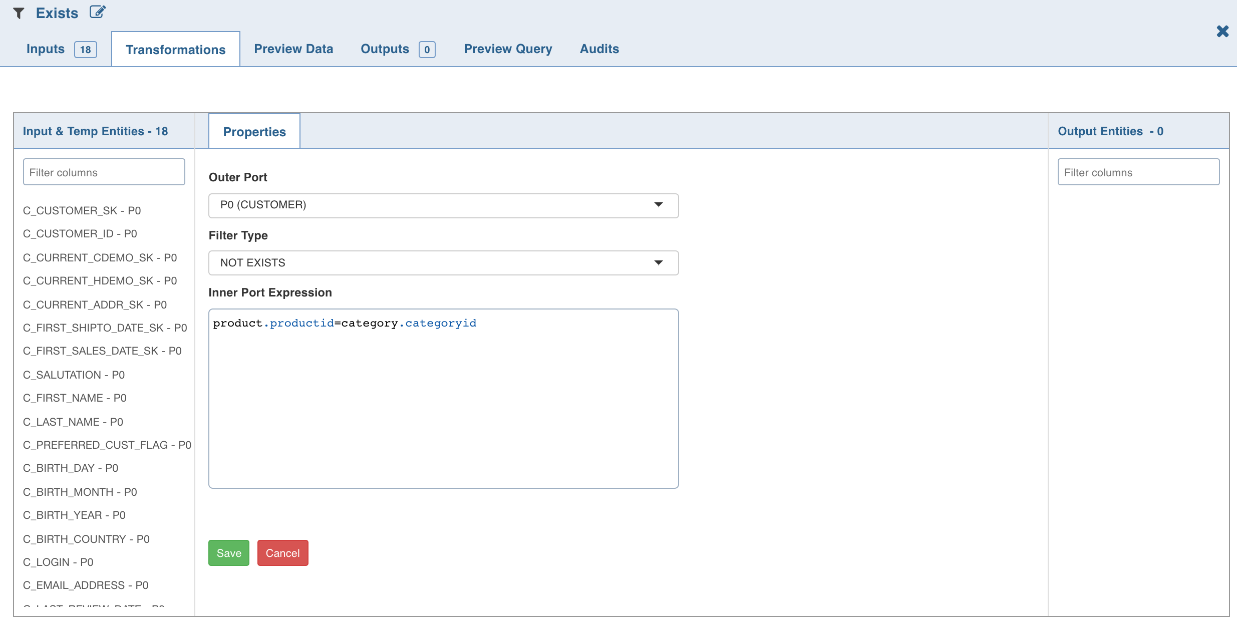
NOTE: Disjuncts, Relational operators other than equals (=), and Complex subquery predicates (like column1+column2 = 100) are not supported.

Custom Transformation

You can add custom transformation logic which cannot be fulfilled by any of the out-of-the-box transformation nodes. This is currently supported for only SPARK execution engine.

Prerequisite

Perform the following:

Navigate to the IW_HOME/opt/infoworks/conf/conf.properties file.
Set the extension path in the user_extensions_base_path configuration. For example, user_extensions_base_path=/opt/infoworks/extensions/.
Ensure that the Infoworks user has write access to the folder.
Restart the UI and Data Transformation services.

Creating Custom Transformation

Implement the SparkCustomTransformation API with a class which has a null constructor. For example, SparkCustomTfmSample.java in IW_HOME/examples/custom-transformation in the Infoworks edge node. You can modify this example java class with the specific transformation requirements. The interfaces to be implemented are packaged in extensions-1.0.jar which you must import in the project. The extensions-1.0.jar is packaged and available with the Infoworks package in the IW_HOME/lib/dt/api/java folder.
Create a jar for the above project.
Upload the jar (and any external dependencies such as Pheonix jars) to a folder in the Infoworks edge node. For example, /home/pivottransformation/. Jars related to Hadoop, spark etc, will already be available on the Infoworks classpath and hence, not required to be placed in this folder.

Registering Custom Transformation

Navigate to Admin > External Scripts > Pipeline Extensions.
Click Add An Extension.

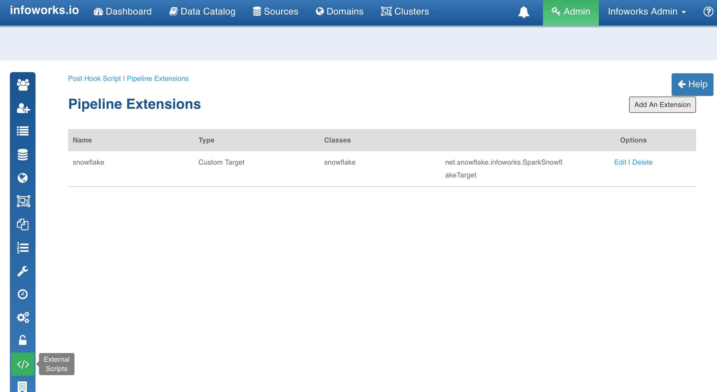
In the Add Pipeline Extension page, enter the following details:

Extension Type: Choose Custom Transformation.
Name: A user-friendly name for the group of transformations under one project. For example, SampleExtension.
Folder Path: The path to the folder where the jars have been uploaded. For example, /home//pivottransformation/.
Classes: The classes implementing the SparkCustomTransformation API which must be available as transformations within Infoworks.
Alias: A user-friendly alias name for the transformations. For example, Sample.
ClassName: A fully qualified class name. For example, io.infoworks.awb.extensions.sample.SparkCustomTfmSample.
You can click Add to add multiple pairs of Alias and Class Names.

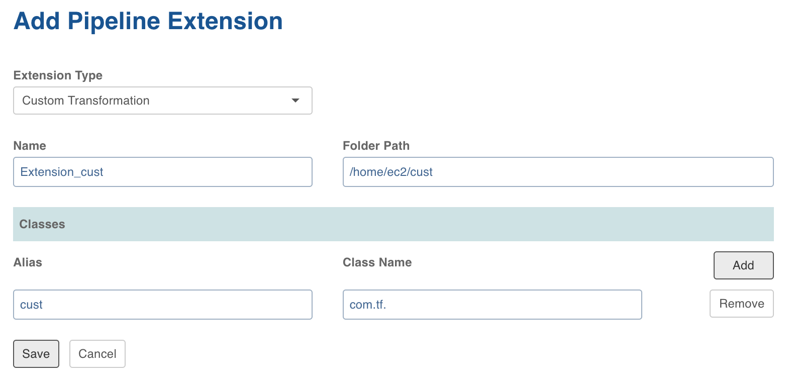
Click Save. Once extension is added successfully, the above transformations will be available in Spark pipeline custom transformations node.

Adding Custom Transformation to Domain

Navigate to Admin > Domains.
Click the Manage Artifacts button for the required domain.
Click the Add Pipeline Extensions button in the Accessible Pipeline Extensions section.
Select the Custom Transformation to be made accessible in the domain.

Using Custom Transformation

Following are the steps to apply Custom Transformation node in pipeline:

Open the pipeline editor, drag and drop Custom Transformation and link it with the dependent parent nodes.
Double-click Custom Transformation and click Edit Properties.
In the Properties page, select the appropriate Extension Name and Extension Class from the respective drop-down lists.
Enter a Key and Value which will be added to the transformation node and will be available via UserProperties class from the public void initialise Context(SparkSession sparkSession, UserProperties userProperties, ProcessingContext processingContext) API.
Click Save.

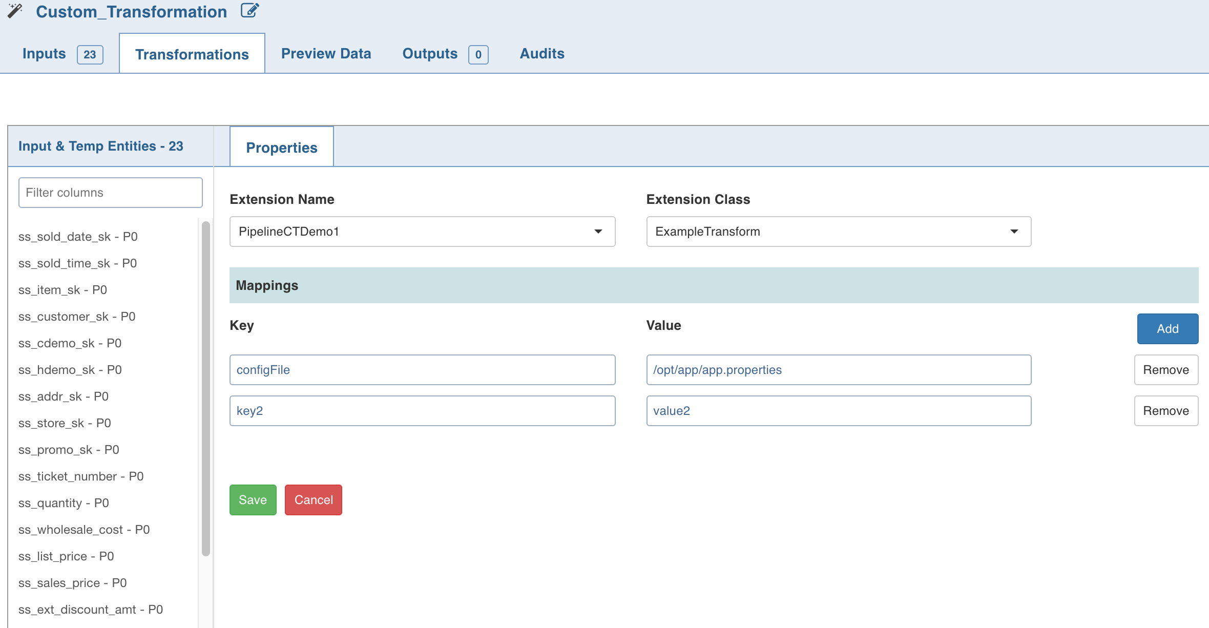
NOTE: When using custom transformation, the output columns must be manually added.

Python Custom Transformation

Data Transformation supports writing custom transformations in Python. This can be used to create custom transformations that can be executed as a part of pipelines to allow integration with proprietary or third party libraries.

Creating Python Custom Transformation

Install the python package in IW_HOME/lib/dt/api using the following command: python -m easy_install <path_for_api-1.0.egg>
Write the custom transformation logic by implementing the Python API CustomTransformation. To import, add the following statement to the Python custom logic: from api.custom_transformation import CustomTransformation
Example for custom transformation is available at /opt/infoworks/examples/custom-transformation/python/sample-code/custom_transformation_example.py
Create .egg extension file for the python project.

NOTE: Use the Java APIs to apply transformation on the input datasets. Internally, py4j is used to communicate to Python custom logic. And, all the provided input data frames are in Java Object form.

Registering Python Custom Transformation

Navigate to Admin > External Scripts > Pipeline Extensions.
Click Add An Extension.

In the Add Pipeline Extension page, enter the following details:

Extension Type: Select Custom Transformation.
Execution Type: Select Python.
Name: A user-friendly name for the group of transformations under one project. For example, SampleExtension.
Folder Path: The path to the folder where the .egg file for the python project is saved. For example, /home/transformation/cust.egg.
Classes: The classes implementing the SparkCustomTransformation API which must be available as transformations within Infoworks.
Alias: A user-friendly alias name for the transformations. For example, Sample.
ClassName: A fully qualified class name in the <python_package>.<python_module>.<class_name> format. For example, io.infoworks.awb.extensions.sample.SparkCustomTfmSample.
You can click Add to add multiple pairs of Alias and Class Names.

NOTES:

Py4j and Pyspark packages must be installed on Python.
Custom transformation with Python runtime is only supported from Python v2.7 onwards.

Configurations

Add dt_scoket_port_range configuration in the pipeline advanced configuration to provide available port range (which will be internally used for socket communication). For example, 25810 : 25890. The default range is 25400 to 25500.
Add dt_socket_max_tries in pipeline advanced configuration to set the maximum number of tries to establish the socket communication. For example, 8. The default value is 10.

NOTE: To execute python scripts, a python executable from the PYSPARK_PYTHON path is used by default.

Pivot

The Pivot node is used to convert data from rows to columns.

Following is a sample table to be pivoted:

orders.order_id	orders.cust_id	orders.prod_id
50001	SMITH	10
50002	SMITH	20
50003	ANDERSON	30
50004	ANDERSON	40
50005	JONES	10
50006	JONES	20
50007	SMITH	20
50008	SMITH	10
50009	SMITH	20

The count for orders grouped by cust_id pivoted on prod_id is as follows:

cust_id	prod__10	prod__20	prod__30	prod__40
ONES	1	1	NULL	NULL
ANDERSON	NULL	NULL	1	1
SMITH	2	3	NULL	NULL

Following are the steps to apply Pivot node in pipeline:

Connect the source node to the Pivot node.
Double-click the Pivot node. The properties page is displayed.
Click the Configurations tab and click Edit Configurations.
Select the column to be pivoted, enter the pivot values and click Save.

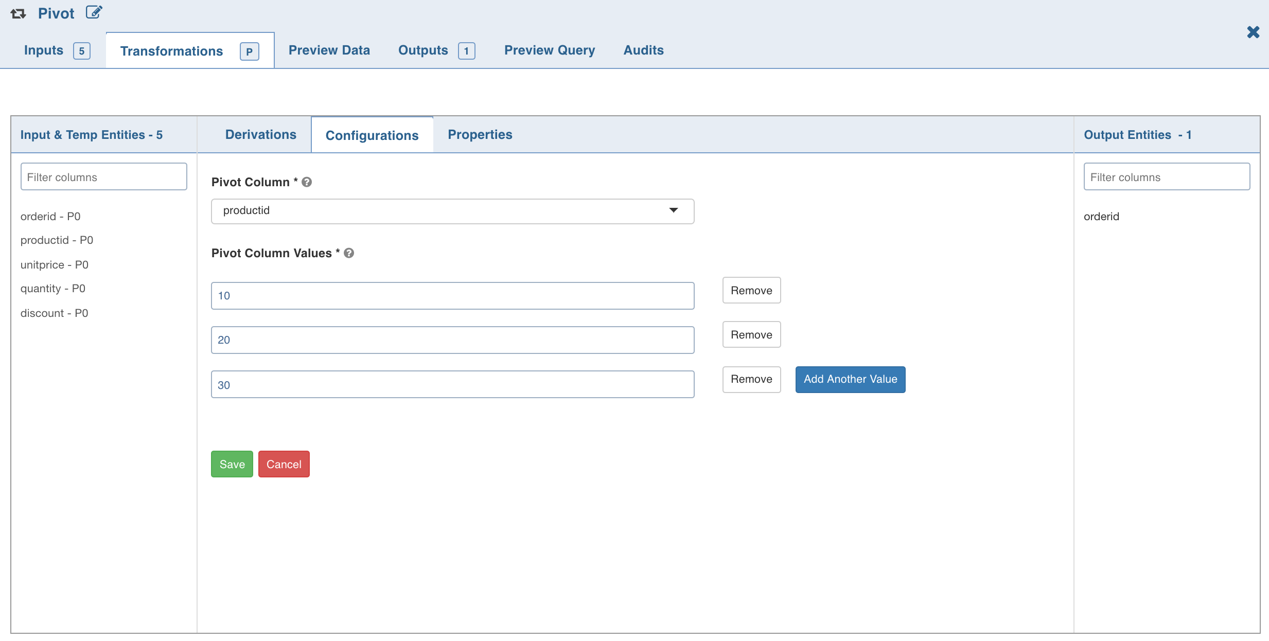
Click the Properties tab and click Add Group By.
Select the group by columns, enter the column name and click Save.

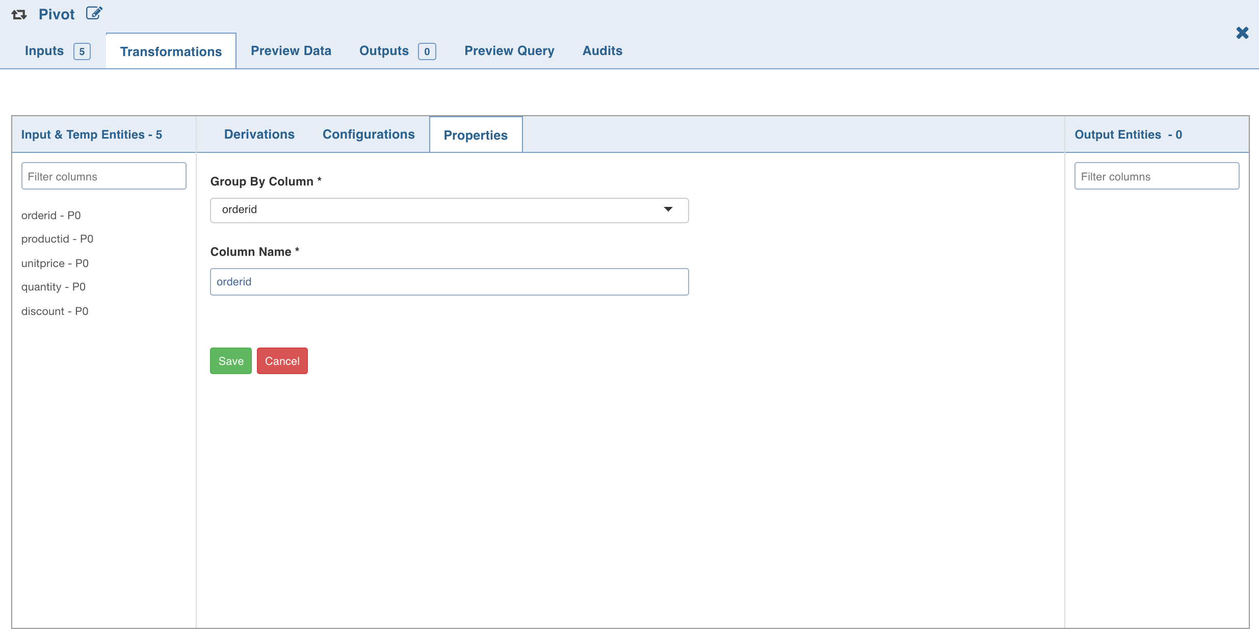
Click Add Aggregate, select the aggregate operation, aggregate column and click Save. The columns are added automatically based on the pivot values; these names can be overridden.
Click the Preview Data tab to view the updated data.

Unpivot

The Unpivot node is used to convert data from columns to rows. You can select one or more columns to be unpivoted.

Connect the source node to the Unpivot node.
Double-click the Unpivot node. The properties page is displayed.
Click the Properties tab and click Edit Properties.
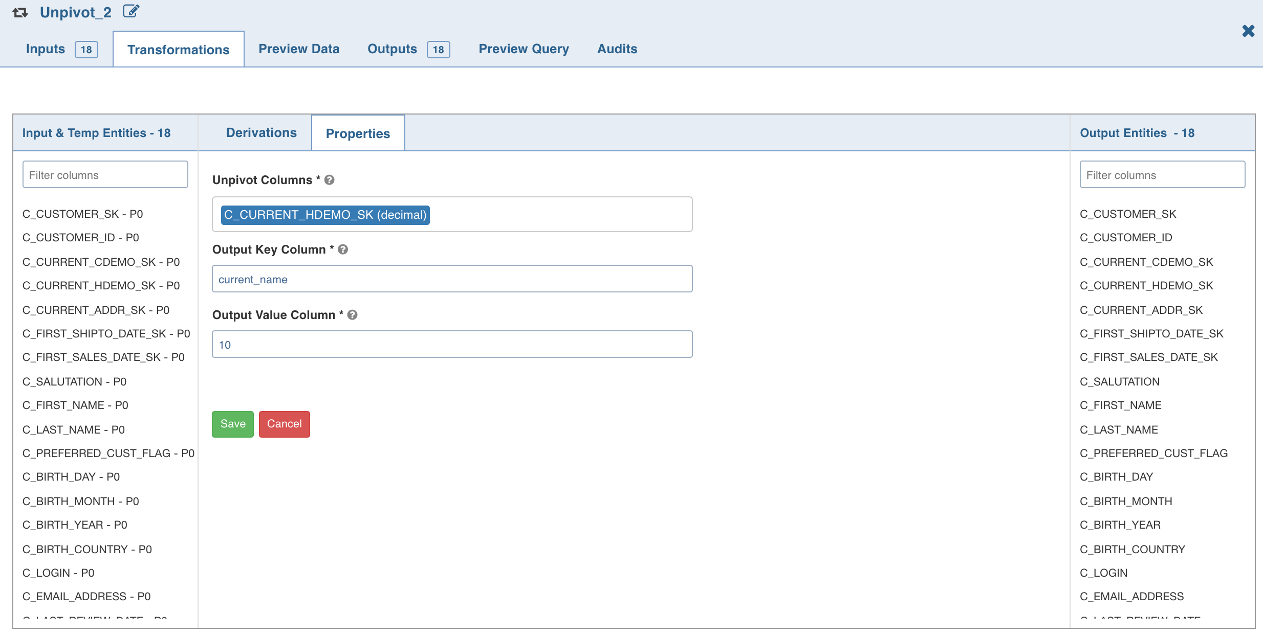
Enter the following details and click Save:
Unpivot Columns: List of columns to be unpivoted. The columns selected will be removed from data and two new columns will be added to the dataset. NOTE: All the unpivot columns must have the same datatype.
Unpivot Key: the names of the selected unpivot columns.
Unpivot Value: the corresponding values of the selected unpivot columns.
Click the Preview Data tab to view the updated data.

Target

For details on the Target node and types of targets supported, see Pipeline Targets.

Last updated on