Introduction
NOTE: Infoworks DataFoundry does not support Cube in HDInsight 3.6 version.
Infoworks Cube helps the user perform multidimensional analysis (hypercube) of data in real time. The user can perform OLAP operations like drill down, roll up, slice and dice on billions of records in interactive querying speeds.
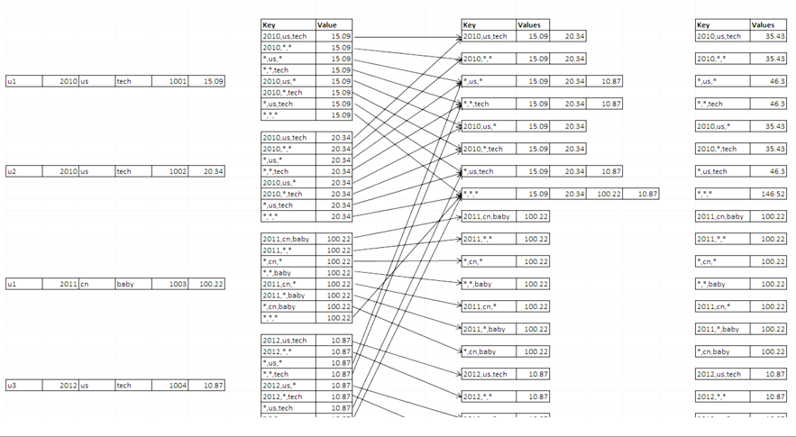
For example, if there are several records stored in tables that represent a relational structure, when the data volume grows very large (10+ or even 100+ billions of rows), a question like "how many units were sold in the technology category in 2010 on the US site?" will produce a query with a large table scan and a long delay to get the answer. Since the values are fixed each time the query is run, it makes sense to calculate and store those values for further usage. This technique is called Relational to Key-Value (K-V) processing. The process will generate all the dimension combinations and measured values shown in the example below, at the right side of the diagram. The middle columns of the diagram, from left to right, show how data is calculated by leveraging MapReduce for the large-volume data processing.
Relational to Key-Value (K-V) Processing - Illustration

Cube Engine is based on this theory and leverages the Hadoop ecosystem to do the job for huge volumes of data. It follows this process:
- Read data from Hive (which is stored on HDFS).
- Run MapReduce jobs to pre-calculate.
- Store cube data in HBase.
- Serve data through Query Engine for aggregation queries.
Many technologies over the past few years have used the same theory to accelerate analytics. These technologies include:
- Methods to store pre-calculated results to serve analysis queries.
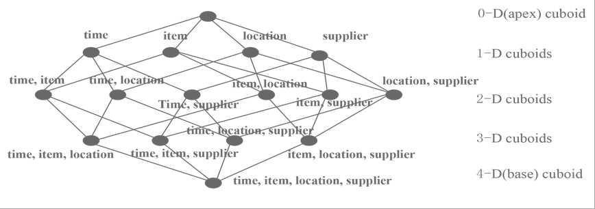
- Generate cuboids for each level with all possible combinations of dimensions.
- Calculate all metrics at different levels. The following figure shows the cuboid topology.
Cuboid Topology
When data volume increases, the pre-calculation processing becomes impossible, even with powerful hardware. However, with the benefit of distributed computing power, calculation jobs can leverage hundreds of thousands of nodes. This allows Cube engine to perform these calculations in parallel and merge the result, thereby significantly reducing the processing time.
Features
- Extremely fast OLAP engine at scale: It is designed to reduce query latency on Hadoop for billions of rows of data.
- Interactive query capability: Users can interact with Hadoop data at sub-second latency - better than batch queries for the same dataset.
- ANSI SQL on Hadoop: Supports most ANSI SQL query functions over JDBC/ODBC.
- Star and Snowflake Cubes: Design Star and Snowflake Cubes with ease.
- Incremental refresh of Cubes: Incrementally add data to cube.
- Seamless integration with BI Tools: Integrates with business intelligence tools such as Tableau and third-party applications.
- Multiple ways to access: Accesses data on BI tools like Tableau using ODBC or directly consume data through JDBC / Java Library / HTTP REST API.
- Aggregation Groups: Improved cube build performance using information about the data and queries/reports that will be run against the cube.
- Augment data: Derives new fact and dimensions specifically for the cube.
- Clone: Clones cube designs and works on top of that to save a lot of design time.
- Easy-to-use: Web interface is easy-to-use which can manage, build, and monitor cubes.
Fact and Dimension Tables
Cubes are created using two types of tables that must be dragged into the Cube Editor Page.
- Fact Tables: A fact table is the central table in a star schema of a data warehouse. A fact table stores quantitative information for analysis and is often denormalized.
- Dimension Tables: A dimension table stores data about the ways in which the data in the fact table can be analyzed.
The fact table consists of two types of columns:
- Foreign keys column allows joins with dimension tables.
- Measures columns contain data that is being analyzed. Example:
If a company sells products to customers, every sale is a fact that happens, and the following fact table is used to record these facts.
Example Fact Table
| Time ID | Product ID | Customer ID | Unit Sold |
|---|---|---|---|
| 4 | 17 | 2 | 1 |
| 8 | 21 | 3 | 2 |
| 8 | 4 | 1 | 1 |
We can now add a dimension table about customers.
Example Dimension Table
| Customer ID | Name | Gender | Income | Education | Region |
|---|---|---|---|---|---|
| 1 | Brian Edge | M | 2 | Masters | San Jose |
| 2 | Fred Smith | M | 3 | Graduate | San Francisco |
| 3 | Sally Jones | F | 1 | Masters | San Diego |
In this example, the Customer ID column in the fact table is the foreign key that joins with the dimension table. By following the links, you can see that row 2 of the fact table records the fact that customer 3, Sally Jones, bought two items on day 8. The company would also have a product table and a timetable to determine what Sally bought and exactly when. When building fact tables, there are physical and data limits. The ultimate size of the object and access paths should be considered. Adding indexes can help with both. However, from a logical design perspective, there should be no restrictions. Tables should be built based on current and future requirements, ensuring that there is as much flexibility as possible built into the design to allow for future enhancements without having to rebuild the data.
Aggregation Groups

Using information about the queries or reports, the cube build performance can be further improved by using Aggregation Groups and prune the cube lattice structure to perform calculations on an optimized set of dimensions. For example, consider the case where all queries we want to run against the above cube involve grouping by item. Then there is no need to calculate aggregations of combinations which do not contain the item in the above lattice. In this example, there is no need to calculate aggregations for groups <time, location>, <time, supplier> and so on, since they do not contain the item dimension.
Types of Dimensions
A dimension can belong to one of the following five types of aggregation groupings:
- Normal Dimensions: Normal dimensions are used to calculate all possible values of the measures for combinations of cube lattice on the columns of these dimensions. Queries on the cube may or may not group by any of these columns.
- Derived Dimensions: Derived dimension is a column on lookup table that can be deduced from another dimension (usually its corresponding PK). For example, UserID -> [Name, Age, Gender], if Name, Age, and Gender are made as derived dimensions, then they can be deduced from primary key UserID. In dimension tables, by default columns except join and normal dimensions are treated as derived dimension.
- Hierarchy Dimensions: Hierarchy Dimensions are the dimensions that form a "contains" relationship where parent column is required for child columns to make sense. For example, Year -> Month -> Day; Country -> City. Hierarchy dimensions are used to calculate the values of the measures for only combinations of cube lattice where "contains" relationship exists on columns of these dimensions.
- Mandatory Dimensions: Mandatory dimensions are used to calculate the values of the measures for only combinations of cube lattice with columns of these dimensions. Queries on the cube must group by the columns of these dimensions.
- Joint Dimensions: Joint dimensions calculate the values of the measures for only combinations of cube lattice with all columns of each set of joint dimensions. Queries on the cube must group either all or none of the columns of every member of a joint set. A dimension can belong to more than one aggregation group. This is especially helpful when we can segregate the queries into different groups. Continuing from the previous example, if there was a smaller set of queries which did not group by item dimension, but grouped by location and supplier, we can have another aggregation group with just location and supplier in a joint dimension set.
All dimensions must be an entry (any type) in at least one aggregation group, however, a single aggregation group need not contain all dimensions.